Mixed Precision Training from Scratch
To really understand the whole picture of Mixed Precision Training, you need to go down to the CUDA level. Staying in Pytorch land can only get you so far:
# Just because you import, doesn't mean you understand.
from torch.cuda.amp import autocast, GradScaler

scaler = GradScaler()
for input, target in data:

    # What is happening here?
    with autocast(device_type='cuda', dtype=torch.float16):
        output = model(input)
        loss = loss_fn(output, target)

    # ...and here?
    scaler.scale(loss).backward()
    scaler.step(optimizer)
    scaler.update()
While torch.cuda.amp offers a seamless way to apply mixed precision training,
it also hides away the most important details. Especially how it makes your model run faster.
The answer, as the library’s name suggests, lies in CUDA.
I decided to rewrite mixed precision training from scratch, going down to the CUDA level, and write this guide. I hope this will help you really understand mixed precision training.
What is Mixed Precision Training?
Mixed precision training is training neural nets with half-precision floats (FP16). This means all of our model weights, activations, and gradients during our forward and backward pass are now FP16, instead of single-precision floats (FP32). Now our memory requirement is halved! Unfortunately, just doing this causes issues with our gradient updates:
for p, grad in zip(parameters, grads): # {p,grad}.dtype = FP16
    update = -lr * grad # update.dtype = FP16
    p.data += update # FP16 += FP16
Since grad is now FP16, it can become too small to be represented in FP16
(any value smaller than 2^-24). When the gradient is less than 2^-24, it underflows to 0 and makes update = 0, causing
our model to stop learning.
Remember, we also made parameters FP16 too. So even if we somehow preserved update to express the too-small-for-FP16
values, adding it to an FP16 tensor like p will cause no change in our weight values.
FP16 sacrifices numerical stability (fancy word for over/underflowing easily) for reduced memory footprint. So how does Mixed Precision Training overcome this trade-off? As the original paper outlines, it offers three solutions.
Let’s go through them one by one, grounding each concept by using it train a simple 2-layer MLP on MNIST.
1. Loss Scaling
Before revealing the answer, it’s often more useful to provide the intuition first. What exactly are our gradient values, and how many of them are outside of this FP16-representable range?
We can visualize this by training our neural net using good ol’ FP32, and plotting a histogram of gradients by their exponent values. Here is ours, modified to demonstrate this concept:
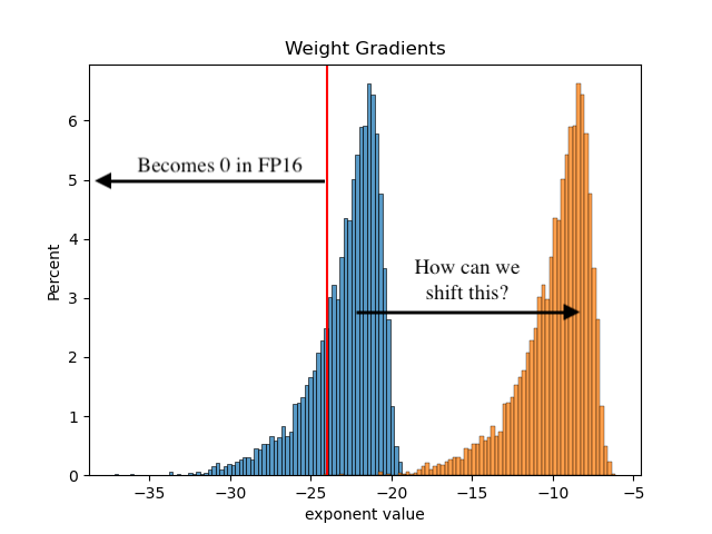
When we convert our gradients to FP16, all the gradients left of the red line will underflow. How can we fix this?
Mixed precision training does it in the simplest way possible: by shifting the gradients to the right. We do this through multiplying the gradients by a constant scale factor, resulting in the orange scaled gradients.
You might ask: why is this called loss scaling and not gradient scaling? The reason is that mixed precision training achieves the same effect by scaling just the loss, before starting backprop. Then the chain rule takes over, ensuring all gradients with respect to the loss are scaled too. It’s also more efficient to scale the loss (a scalar), than to scale all gradients (tensors).
Before moving on, it’s important to note that not all neural nets require loss scaling. Our 2-layer MLP’s actual gradient histogram proves this:
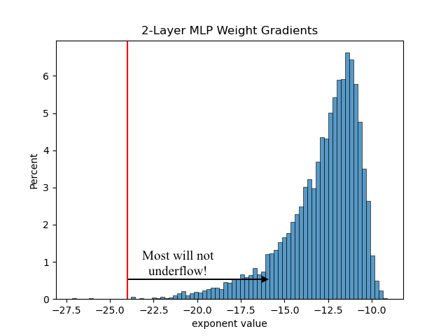
I still implemented loss scaling for pedagogical reasons, and because it was dead simple to do so:
loss = F.cross_entropy(logits, y) # end of forward pass

# Start manual backward pass.
# Cast logits to fp32 before softmax to prevent underflow
dlogits = F.softmax(logits, 1, dtype=torch.float32)
dlogits[range(n), y] -= 1
dlogits /= n

# loss scaling
# note: we multiply dlogits, instead of loss, by scale. This is because
#   we are doing backprop manually. The first gradient is dlogits, and the
#   scale will propogate through all gradients.
dlogits *= scale
dlogits = dlogits.to(torch.float16) # no underflow occurs!
The gradient update adds an unscaling step:
for p, grad in zip(parameters, grads):
    update = -lr * (grad.to(torch.float32) / scale) # fp32 upcast, then unscale
    p.data += update # update is fp32, but p is still fp16. Hmm...
It’s important that we convert the gradients to FP32 before we unscale, can you guess why? :)
2. FP32 Master Copy of Weights
Updates no longer underflow in FP32. But when adding them to our FP16 weights, updates will underflow again because they are downcasted to FP16 before the addition. All our loss scaling work would have been for nothing!
Mixed precision training keeps an FP32 master copy of weights to solve this. We still use FP16 weights for our forward and backward pass, but at the optimizer step, we update the FP32 master weights:
# Define master weights. Notice the fp32 dtypes.
# linear layer 1
m_W1 = torch.rand((n_embd, n_hidden), dtype=torch.float32)
m_b1 = torch.rand(n_hidden, dtype=torch.float32)

# linear layer 2
m_W2 = torch.rand((n_hidden, num_classes), dtype=torch.float32)
m_b2 = torch.rand(num_classes, dtype=torch.float32)

parameters = [m_W1, m_b1, m_W2, m_b2]

for i, (x,y) in enumerate(dloader):

    # Convert to fp16 for forward and backward pass
    W1, b1, W2, b2 = m_W1.half(), m_b1.half(), m_W2.half(), m_b2.half()

    # (omitted forward/backward pass code that uses the fp16 weights)

    grads = [dW1, db1, dW2, db2]
    for p, grad in zip(parameters, grads): # updating fp32 master weights
        p.data += -lr * (grad.to(torch.float32) / scale)
Because we are keeping an additional FP32 copy of weights + the FP16 weights, our model memory requirement actually increases by 50% compared to single precision training (only FP32 weights required). For training however, memory consumption is dominated by activations and gradients, especially for large neural nets with many layers and huge batch sizes.
I replicated this phenomenon for our tiny 2-layer MLP:
$ python train.py false
device: cuda, mixed precision training: False (torch.float32)
model memory: 26.05 MB
act/grad memory: 1100.45 MB
total memory: 1126.50 MB
...
$ python train.py true
device: cuda, mixed precision training: True (torch.float16)
model memory: 39.08 MB
act/grad memory: 563.25 MB
total memory: 602.33 MB
While model memory does increase by 50%, our activations decrease by half. Overall, total memory is nearly halved.
3. Mixed Precision Arithmetic
Our gradient updates are now numerically stable. But there still remains one more source of numerical instability.
Technically, it’s not one. Pretty much every other operation we do in our model (matmult, softmax, relu, etc.) can be unstable in FP16. It’s so unstable that even PyTorch refuses to do them:
>>> F.softmax(a,1)
tensor([[0.2598, 0.7402],
        [0.8864, 0.1136]])
>>> F.softmax(a.half(),1)
Traceback (most recent call last):
  File "<stdin>", line 1, in <module>
  File "/Users/peter/miniconda3/envs/torch/lib/python3.10/site-packages/torch/nn/functional.py", line 1843, in softmax
    ret = input.softmax(dim)
RuntimeError: "softmax_lastdim_kernel_impl" not implemented for 'Half'
So how does my code run? CUDA saves the day here:
>>> F.softmax(a.half().cuda(),1)
tensor([[0.2598, 0.7402],
        [0.8864, 0.1136]], device='cuda:0', dtype=torch.float16)
Just like softmax, CUDA offers numerically stable versions of popular deep learning ops for FP16. It does this through mixing arithmetic precisions. E.g. For matmults, or vector dot-products, the multiplication is done in FP16 but the partial products are accumulated as FP32.
Let’s go down to CUDA land and see this in action. I wanted to demonstrate this as simply as possible, so I reimplemented the matmult operator with cuBLAS:
// C = alpha AB + beta C
void matmult(torch::Tensor A, torch::Tensor B, torch::Tensor C,
    bool transpose_A, bool transpose_B, float alpha, float beta) {

    // Additional code omitted for clarity.

    if (A.dtype() == torch::kFloat32) {
        cublasGemmEx(get_handle(), op_B, op_A, n, m, k, &alpha,
                     B.data_ptr<float>(), CUDA_R_32F, B.size(1),
                     A.data_ptr<float>(), CUDA_R_32F, A.size(1),
                     &beta, C.data_ptr<float>(), CUDA_R_32F, C.size(1),
                     CUBLAS_COMPUTE_32F, CUBLAS_GEMM_DEFAULT_TENSOR_OP);
    } else if (A.dtype() == torch::kFloat16) {
        cublasGemmEx(get_handle(), op_B, op_A, n, m, k, &alpha,
                     B.data_ptr<at::Half>(), CUDA_R_16F, B.size(1),
                     A.data_ptr<at::Half>(), CUDA_R_16F, A.size(1),
                     &beta, C.data_ptr<at::Half>(), CUDA_R_16F, C.size(1),
                     CUBLAS_COMPUTE_32F, CUBLAS_GEMM_DEFAULT_TENSOR_OP);
    }
}
First, we call cublasGemmEx with different parameters based on the precision type (this is how PyTorch
does it too in essence, through dispatching).
For FP16 tensors, we set the cudaDataType as CUDA_R_16F,
which will read and write FP16 results. However, by specifying
the cublasComputeType as CUBLAS_COMPUTE_32F,
the dot-products are accumulated as FP32.
Doing this mixed precision arithmetic allows us to retain numerical stability in our FP16 matmults.
In my final code, I load and call cuBLAS through a PyTorch extension:
# load matmult CUDA call as extension
mpt = load(name='mixed_precision_training', sources=['main.cpp', 'matmult.cu'],
           extra_cuda_cflags=['-O2', '-lcublas'])

# (omitted...)

mpt.matmult(x, W1, a1, False, False, 1.0, 1.0) # a1 = x @ W1 + b1
# Sanity check - exact match with PyTorch's FP16, numerically stable matmults
cmp('a1', a1, x @ W1 + b1)
The Secret Sauce: Tensor Cores
Now that we’ve made it down to CUDA land, I can finally show you why using FP16 for our weights and activations
magically makes our model train faster. It’s because calling cublasGemmEx with FP16 datatypes (+ few other
rules) activates Tensor Cores:
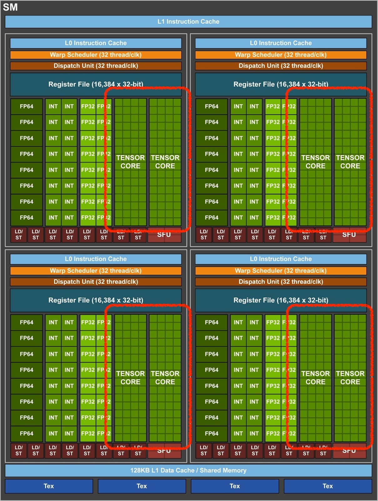
Starting with Volta GPUs (like the V100 that I’m using), FP16 matmults are accelerated from a hardware level using Tensor Cores. They make them about an order of magnitude faster than FP32 matmults (taken from the V100 microbench report):
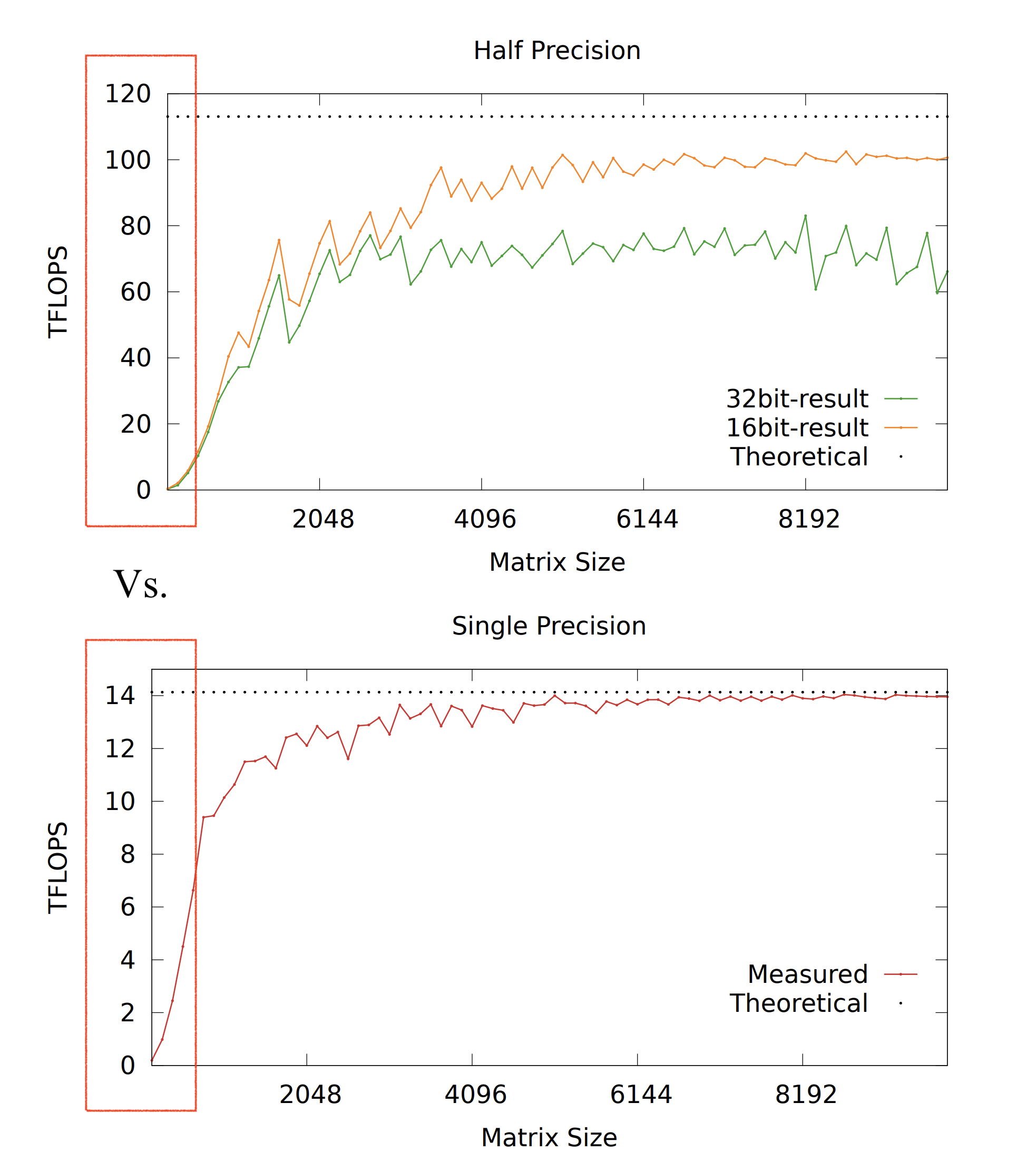
With the secret sauce that is Tensor Cores, mixed precision training achieves higher training throughput. Thanks to them, my custom matmults are faster during both the forward and backward pass, doubling the training speed for our 2-layer MLP:
$ python train.py false
device: cuda, mixed precision training: False (torch.float32)
model memory: 26.05 MB
act/grad memory: 1100.45 MB
total memory: 1126.50 MB
1: loss 2.327, time: 139.196ms
2: loss 2.237, time: 16.598ms
3: loss 2.175, time: 16.179ms
4: loss 2.117, time: 16.206ms
5: loss 2.058, time: 16.187ms
6: loss 2.006, time: 16.207ms
7: loss 1.948, time: 16.304ms
avg: 16.280ms
$ python train.py true
device: cuda, mixed precision training: True (torch.float16)
model memory: 39.08 MB
act/grad memory: 563.25 MB
total memory: 602.33 MB
1: loss 2.328, time: 170.039ms
2: loss 2.236, time: 8.513ms
3: loss 2.176, time: 8.440ms
4: loss 2.117, time: 8.356ms
5: loss 2.059, time: 8.133ms
6: loss 2.006, time: 8.370ms
7: loss 1.948, time: 8.402ms
avg: 8.369ms
Wow, mixed precision training is 2x faster and uses 2x less memory!
Wrap-up
If you made it this far, you’ve now seen everything that mixed precision training has to offer. It can be reduced to training with lower precision tensors to decrease memory usage, while compensating for the numerical instability through three approaches - loss scaling, fp32 master weights, and mixed precision arithmetic.
Most importantly, you saw the CUDA code that activates hardware-accelerated matmults through Tensor Cores. This is what makes GPUs go brrr. Now you understand why mixed precision training is basically a necessity for training larger and larger neural nets: it is because we want to exploit these Tensor Cores.
Thanks for reading, and I hope now you really understand mixed precision training.
You can check out my full implementation on Github.